Quantum GIS


 (41 votes, average: 3.90 out of 5)
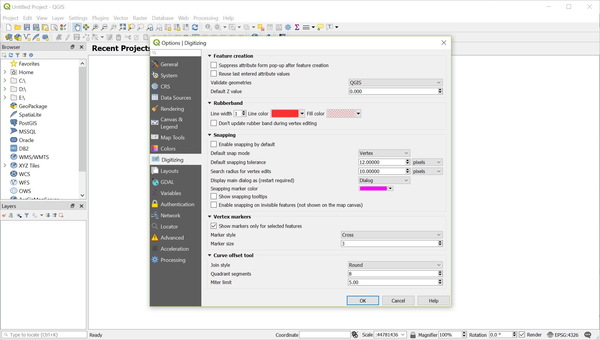
About Quantum GIS
If you do any work with maps that goes beyond drawing pins on Google Maps, Quantum GIS is probably the application you end up using. It’s a full desktop geographic information system, free and open source, with a feature surface that overlaps significantly with ArcGIS and a few specific corners where it actually goes further. Cartographers, urban planners, environmental researchers, archaeologists, transport analysts, and anyone else who needs to read, edit, analyze, and publish spatial data ends up here sooner or later.
The application reads pretty much any geospatial format that has ever shipped a public driver. Shapefiles, GeoPackage, GeoJSON, KML, GPX, GML, MapInfo TAB, AutoCAD DXF, raster formats like GeoTIFF, ECW, JP2, ASCII grids, MrSID, plus direct connections to PostGIS, SpatiaLite, Oracle Spatial, and Microsoft SQL Server spatial extensions.
Web services come in through WMS, WMTS, WFS, WCS, and a growing set of vector tile and ArcGIS REST connectors. The point isn’t completeness for its own sake. It’s that you can open whatever spatial data lands on your desk without first converting it to something the application understands.
QGIS, the modern name, is technically what the project goes by now. Quantum GIS was the original name and it stuck in a lot of training materials, course syllabi, and search habits.
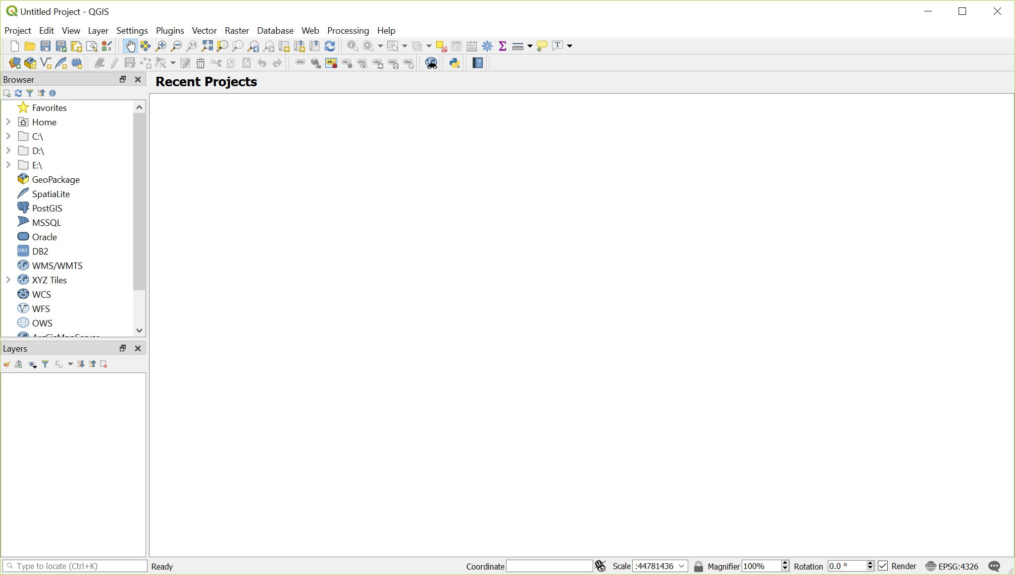
The layered approach to spatial data
Everything in the application happens through layers. You add data as a layer, the layer sits in a stack, and the map canvas renders the stack from bottom to top. Vector layers carry features with attributes. Raster layers carry pixel values across a defined extent. Each layer has its own coordinate reference system, its own styling rules, and its own attribute table.
The on-the-fly reprojection is where this gets useful. You can mix layers in different projections in the same map and the application handles the transformation automatically for display. That sounds basic but it’s the kind of thing that breaks workflows in tools without it, since you’d otherwise need to reproject every dataset to match a chosen base projection before adding it.
The downside is real. On-the-fly reprojection eats CPU on dense vector layers, and complex transformations between projections can produce subtle accuracy issues at edges. For final cartographic output most users reproject explicitly to a common CRS and turn the on-the-fly handling off.
Vector editing and topology
Editing vector layers is where the application competes most directly with commercial alternatives. You can digitize new features, snap to existing geometry, split or merge features, and manage attributes through the table view or a custom form. Topology checking flags overlaps, gaps, and dangling nodes across layers, which matters when you’re building a polygon coverage that has to be gap-free.
The snapping toolbar is configurable to the point of overkill. You can snap to vertices only, segments only, both, with tolerances measured in pixels or map units, and with per-layer overrides.
Once you’ve set it up for a specific dataset, the editing workflow is fast. Setting it up is the hump. For CAD-style precision work where coordinate input matters more than spatial topology, a dedicated CAD viewer like DraftSight handles a different but adjacent use case.
The processing toolbox and geoalgorithms
The Processing toolbox is the unsung core of the application. Hundreds of algorithms, organized by category, covering vector analysis, raster analysis, geometry operations, network analysis, interpolation, terrain analysis, and conversions. Most algorithms accept any of the standard input formats and produce results as new layers or files on disk.
Behind the scenes the toolbox is a wrapper. It calls GDAL, GRASS GIS, SAGA GIS, and the application’s own native algorithms through a unified interface, which means you get the union of all of those toolsets without switching applications.
The unification isn’t always seamless. Some algorithms have quirky parameter names inherited from GRASS, some expect specific input formats, some fail silently when run on data they don’t like. The error messages have improved but you’ll still hit cases where the only way to debug is to run the underlying tool directly.
The Graphical Modeler lets you chain algorithms into a reusable workflow without writing code. Drag an input, connect it to an algorithm, connect that to the next algorithm, save the model, and it shows up in the toolbox like any other tool. For repeatable analysis pipelines, this is genuinely useful.
Python and PyQGIS
The application is built on Python and exposes essentially everything through a scripting interface called PyQGIS. The built-in Python console lets you query layers, run algorithms, manipulate geometries, and automate batch tasks interactively. Scripts can be saved as toolbox algorithms, called from models, or run from the command line through the headless processing runner.
For users coming from the data science side, the Anaconda distribution plays well with the application’s Python environment, allowing geopandas, shapely, and rasterio workflows to coexist with the GUI when you need both interactive editing and code-driven processing.
The plugin ecosystem is built on the same Python foundation. The official plugin repository hosts hundreds of community plugins covering specific niches the core application doesn’t address. QuickOSM for OpenStreetMap queries, MMQGIS for batch geoprocessing, Profile Tool for elevation profiles, qgis2web for exporting interactive web maps, Time Manager for animating temporal data.
The quality varies. Some plugins are essentially production tools maintained for years, others were a weekend project that hasn’t been updated since.
Database integration and the PostGIS angle
The database side of the application is built around PostGIS, the spatial extension for PostgreSQL. You can connect directly to a PostGIS database, browse spatial tables in the layer browser, edit features in place, and execute SQL through the DB Manager. For multi-user GIS environments where the data lives in a database rather than in files on a shared drive, this is the canonical setup.
SpatiaLite (PostGIS’s SQLite-based cousin) works the same way for single-user databases. GeoPackage is the modern recommendation for file-based spatial storage, since it handles vectors, rasters, and styles in one container without the multi-file mess of shapefiles.
The application can also read directly from cloud-optimized GeoTIFFs and other cloud-native formats over HTTP, which matters for satellite imagery workflows where the file lives in S3 rather than locally.
Print Layout and cartographic output
The Print Layout (formerly Print Composer) is where the application produces presentation-quality maps. It’s a separate window where you arrange map frames, legends, scale bars, north arrows, titles, and annotations on a page of arbitrary size. Export goes to PDF, SVG, or raster image formats.
The cartographic quality matches what serious commercial tools produce. Label placement is configurable down to the level of rule-based collision avoidance, you can apply curved labels along linear features, and the rendering engine handles transparency and blending modes that older GIS software couldn’t. SVG export opens cleanly in Inkscape for hand-tuning if the automatic output isn’t quite right for print.
The atlas feature deserves a specific mention. Atlas mode generates a separate map page for each feature in a coverage layer, automatically filtering and zooming the map frame to that feature. For producing parcel maps, neighborhood profiles, or any series of similar maps with different extents, it replaces what would otherwise be hours of manual repetition.
Where the experience falls short
The learning curve is steep. The interface is dense, the terminology comes from a deep technical tradition, and the documentation while comprehensive assumes a baseline of GIS literacy. New users coming in cold tend to bounce off until they find a tutorial that matches their specific goal, and then they bounce off again the next time they try something new.
Stability under load is better than it used to be but still imperfect. Large raster operations, certain projection edge cases, and some plugin combinations can crash the application without warning. The auto-save and project recovery has improved, but you’ll still want to save manually before kicking off any heavy processing job. Plugin quality is the wild west, which means an unmaintained plugin can drag down an otherwise stable session.
The 3D capabilities work but lag behind dedicated 3D GIS tools. The renderer handles draped imagery on terrain and basic 3D feature extrusion, but for serious 3D analysis you’d reach for something more specialized. Google Earth covers the casual 3D visualization angle for users who don’t need actual analytical capability.
Conclusion
Quantum GIS is the open source application that turned desktop GIS from a niche commercial market into something a graduate student, a small consultancy, or a municipal planning office could realistically adopt without a five-figure license. The depth of the format support, the breadth of the processing toolbox, and the extensibility through Python and plugins put it in the same conversation as commercial alternatives that cost orders of magnitude more.
The audience that gets the most out of the application is users who treat GIS as a working tool rather than a one-off task. Planners producing recurring map series through atlas mode, analysts running repeatable workflows through the graphical modeler, researchers querying spatial databases for specific patterns.
Casual users who need to throw pins on a map and share it will find it overkill, and that’s fair, the application is built for serious spatial work and that’s where it earns its position in the toolkit.
Pros & Cons
- Free and open source with no licensing limits on use, commercial included
- Reads essentially every spatial format through GDAL and OGR drivers
- Processing toolbox unifies GRASS, SAGA, GDAL, and native algorithms
- PyQGIS and the plugin ecosystem extend functionality across hundreds of niches
- Print Layout produces presentation-quality cartographic output with atlas generation
- Direct PostGIS and SpatiaLite integration for database-driven workflows
- On-the-fly reprojection allows mixed-CRS layers in one map
- Steep learning curve for users without prior GIS exposure
- Stability under heavy raster processing or with some plugin combinations remains imperfect
- Plugin ecosystem varies in quality, with many community plugins unmaintained
- 3D viewer is functional but lags behind dedicated 3D tools
- Some processing algorithms inherit awkward parameter conventions from underlying libraries
Frequently asked questions
They're the same project. Quantum GIS was the original name, shortened to QGIS at some point during development. Older tutorials and documentation still use the longer form, which is why both names show up in search results.
Yes, shapefiles are a first-class supported format. Drag the .shp file into the layer panel and the application loads it along with the associated .dbf attribute table and .prj projection file if present.
KML and KMZ files import directly as vector layers. The application can also export to KML for viewing in Google Earth. Round-tripping data between the two is straightforward as long as you keep an eye on coordinate reference systems.
Use the "Extract by Location" or "Clip" algorithm in the Processing toolbox. Select your point layer as input, your polygon layer as the spatial filter, choose the spatial predicate (within, intersects, etc.), and the algorithm produces a new layer containing only the points that match.
Yes through several paths. The DB Manager handles SQL against PostGIS, SpatiaLite, and other connected databases. The Virtual Layer feature lets you write SQL against any loaded vector layer regardless of source format. Both support spatial SQL functions like ST_Intersects and ST_Buffer.
Through GDAL and the native processing algorithms. You can do raster math through the Raster Calculator, terrain analysis (slope, aspect, hillshade) through dedicated tools, supervised classification through plugin extensions, and reprojection or resampling through standard toolbox algorithms.
Most often the cause is a malformed projection definition, a corrupted file header, or an unusually large file that exceeds available memory. Run gdalinfo (included with the application) against the file from the command line to see what GDAL reports. Many crashes traceable to plugins resolve by disabling the plugin and reopening the file.